Image Source
During text processing & information retrieval we often need to find important words in document which can also help us identify what a document is about. tf-idf uses term frequency & inverse term frequency to find this. In this notebook I will briefly discuss tf-idf followed by an implementation of tf-idf on novel ‘Alice’s Adventures in Wonderland’ using tidytext package in R.
Term Frequency
The term frequency of a term t in a document d represent the number of times t occurs in d. So a document with higher term frequency might be more relevant for searched term, but document relevance is not directly related to term frequency for example if we search for term ‘car’ then a document having car 10 times in it may not be 10 times more relevant compared to document with word ‘car’ appearing say only 1 or 2 times.
So TF or Term Frequency can be expressed as log of actual frequency as:
here 1 is added to avoid infinity in case term frequency us 0. if term does not occur in document then we can set tf as 0.
Inverse Term Frequency
If we only use term frequency during text processing then most stop words like the,to,is etc. will get very high tf values which will not be relevant, so we use idf which decreases the weight for commonly used words and increases the weight for words which are actually relevant during information retrieval.
IDF or inverse document frequency is expressed as:
here represents total number of documents in our corpus & represent number of documents which contain term t. Here frequent stop word like ‘the’ will be present in almost all documents making & .
TF-IDF
Combination of tf & idf is measure of how important a word is to a document in a corpus of documents. tf-idf is expressed as:
Note: In tf-idf there is hyphen between tf & idf, don’t confuse this with subtraction, tf & idf are multiplied here.
Finding tf-idf values from novel ‘Alice’s Adventures in Wonderland’
Downloading novel ‘Alice’s Adventures in Wonderland’ from gutenberg.org using gutenbergr package
raw_text <- gutenberg_download(28885) #Alice's Adventures in Wonderland by Lewis Carroll
Alice’s Adventures in Wonderland contains 12 Chapters, I will treat each chapter as a document and find tf-idf across each chapter of novel. Lets drive 3 new features story, line & word from raw_text.
alice <- raw_text %>%
    mutate(story = ifelse(str_detect(text, "CHAPTER"), text, NA)) %>%
    fill(story) %>%
    mutate(story = factor(story, levels = unique(story))) %>%
    mutate(line = row_number()) %>%
    unnest_tokens(word, text)

alice

## # A tibble: 27,586 x 4
##    gutenberg_id  story  line               word
##           <int> <fctr> <int>              <chr>
##  1        28885     NA     1            alice's
##  2        28885     NA     1         adventures
##  3        28885     NA     1                 in
##  4        28885     NA     1         wonderland
##  5        28885     NA     3       illustration
##  6        28885     NA     3              alice
##  7        28885     NA     5       illustration
##  8        28885     NA     7 alice's.adventures
##  9        28885     NA     8      in.wonderland
## 10        28885     NA     9   by.lewis.carroll
## # ... with 27,576 more rows
Lets find most frequent word in novel by sorting words by their frequency
alice %>%
  count(word, sort = TRUE)

## # A tibble: 2,919 x 2
##     word     n
##    <chr> <int>
##  1   the  1676
##  2   and   899
##  3    to   757
##  4     a   649
##  5   she   543
##  6    it   539
##  7    of   523
##  8  said   466
##  9 alice   391
## 10     i   391
## # ... with 2,909 more rows
As most stop words like the, to, a etc. are most frequent in most text corpus we need to remove these to get more relevant words.
Removing stop words
tidy_alice <- alice %>%
    anti_join(stop_words)

## Joining, by = "word"

tidy_alice

## # A tibble: 8,319 x 4
##    gutenberg_id       story  line        word
##           <int>      <fctr> <int>       <chr>
##  1        28885 CHAPTER XII  3635  apostrophe
##  2        28885 CHAPTER XII  3635         153
##  3        28885 CHAPTER XII  3633 parenthesis
##  4        28885 CHAPTER XII  3631         hog
##  5        28885 CHAPTER XII  3631         104
##  6        28885 CHAPTER XII  3629         103
##  7        28885 CHAPTER XII  3627          91
##  8        28885 CHAPTER XII  3624      single
##  9        28885 CHAPTER XII  3624          69
## 10        28885 CHAPTER XII  3622   quotation
## # ... with 8,309 more rows
Words sorted by frequency, here alice is most frequent word followed by queen & time.
tidy_alice %>%
  count(word, sort = TRUE)

## # A tibble: 2,448 x 2
##       word     n
##      <chr> <int>
##  1   alice   391
##  2   queen    73
##  3    time    73
##  4    king    61
##  5    mock    59
##  6  turtle    58
##  7 gryphon    55
##  8  hatter    55
##  9    head    53
## 10  rabbit    49
## # ... with 2,438 more rows
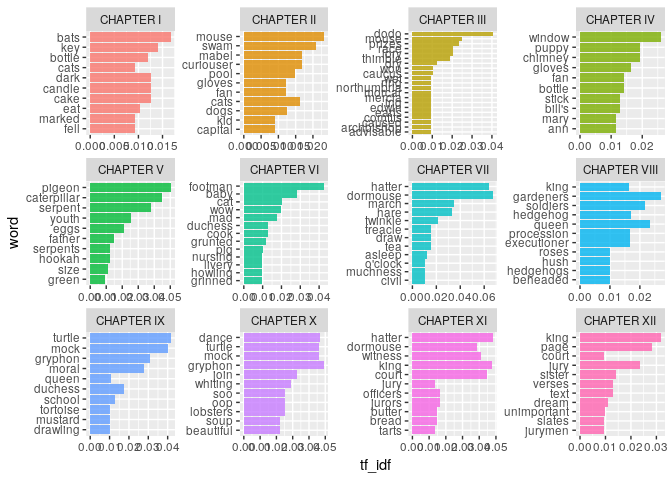
Top 10 words with highest tf-idf values in each Chapter of Alice’s Adventures in Wonderland
tidy_alice %>%
    count(story, word, sort = TRUE) %>%
    bind_tf_idf(word, story, n) %>%
    arrange(-tf_idf) %>%
    group_by(story) %>%
    top_n(10) %>%
    ungroup %>%
    mutate(word = reorder(word, tf_idf)) %>%
    ggplot(aes(word, tf_idf, fill = story)) +
    geom_col(alpha = 0.8, show.legend = FALSE) +
    facet_wrap(~ story, scales = "free") +
    coord_flip()

## Selecting by tf_idf
Lets also check words with highest tf-idf values in alice dataset with stop words included
alice %>%
    count(story, word, sort = TRUE) %>%
    bind_tf_idf(word, story, n) %>%
    arrange(-tf_idf) %>%
    group_by(story) %>%
    top_n(10) %>%
    ungroup %>%
    mutate(word = reorder(word, tf_idf)) %>%
    ggplot(aes(word, tf_idf, fill = story)) +
    geom_col(alpha = 0.8, show.legend = FALSE) +
    facet_wrap(~ story, scales = "free") +
    coord_flip()

## Selecting by tf_idf
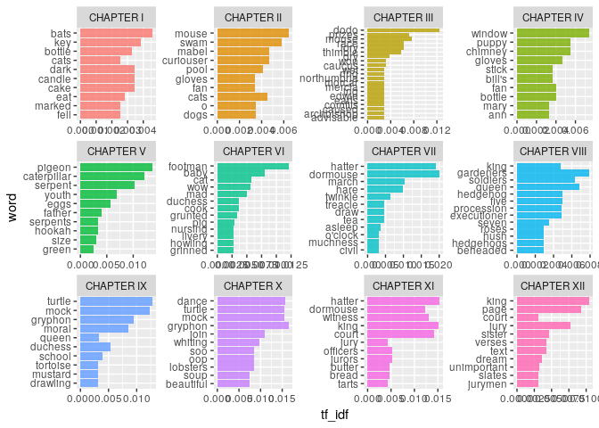
As expected top tf-idf values are not affected by stop words as IDF values of such stop words are very small due to their presence in almost every chapter.
Refrences
- Project Gutenburg, http://www.gutenberg.org/
- Tidy Text Mining with R, https://www.tidytextmining.com/
- Speech & language processing, https://web.stanford.edu/~jurafsky/slp3/
- gutenbergr, https://cran.r-project.org/web/packages/gutenbergr/index.html
Thanks for reading this notebook. In my next notebook I will extend this idea further & use tf-idf values to explore Topic Models.