Image Source
Data description
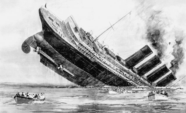
The sinking of the RMS Titanic is one of the most infamous shipwrecks in history. On April 15, 1912, during her maiden voyage, the Titanic sank after colliding with an iceberg, killing 1502 out of 2224 passengers and crew.
In this Notebook I will do basic Exploratory Data Analysis on Titanic dataset using R & ggplot & attempt to answer few questions about Titanic Tragedy based on dataset. Dataset was obtained from kaggle (https://www.kaggle.com/c/titanic/data).
Data Dictionary
| Variable | Definition | Key |
|---|---|---|
| survival | Survival | 0 = No, 1 = Yes |
| pclass | Ticket class | 1 = 1st, 2 = 2nd, 3 = 3rd |
| embarked | Port of Embarkation | C = Cherbourg, Q = Queenstown, S = Southampton |
| sex | Sex | |
| Age | Age in years | |
| sibsp | # of siblings / spouses aboard the Titanic | |
| parch | # of parents / children aboard the Titanic | |
| ticket | Ticket number | |
| fare | Passenger fare | |
| cabin | Cabin number |
Fetching data
Toggle Code button to see steps
knitr::opts_chunk$set(echo = TRUE)
library(dplyr)
library(ggplot2)
library(knitr)
library(kableExtra)

titanic_train<-read.csv('train.csv')
titanic_test<-read.csv('test.csv')
Merging train & test sets for complete Exploratory Analysis
titanic_test$Survived <- NA
titanic <- rbind(titanic_train, titanic_test)
Though we can use merged dataset for EDA but I will use train dataset only for EDA for consistency & simplicity as Survival attribute is missing from test data.
Dataset Preview
These are first few records from titanic dataset.
head(titanic) %>% kable("html") %>%
  kable_styling()
| PassengerId | Survived | Pclass | Name | Sex | Age | SibSp | Parch | Ticket | Fare | Cabin | Embarked |
|---|---|---|---|---|---|---|---|---|---|---|---|
| 1 | 0 | 3 | Braund, Mr. Owen Harris | male | 22 | 1 | 0 | A/5 21171 | 7.2500 | S | |
| 2 | 1 | 1 | Cumings, Mrs. John Bradley (Florence Briggs Thayer) | female | 38 | 1 | 0 | PC 17599 | 71.2833 | C85 | C |
| 3 | 1 | 3 | Heikkinen, Miss. Laina | female | 26 | 0 | 0 | STON/O2. 3101282 | 7.9250 | S | |
| 4 | 1 | 1 | Futrelle, Mrs. Jacques Heath (Lily May Peel) | female | 35 | 1 | 0 | 113803 | 53.1000 | C123 | S |
| 5 | 0 | 3 | Allen, Mr. William Henry | male | 35 | 0 | 0 | 373450 | 8.0500 | S | |
| 6 | 0 | 3 | Moran, Mr. James | male | NA | 0 | 0 | 330877 | 8.4583 | Q |
Data Structure & Summary
str(titanic) #1309 obervations & 12 variables

## 'data.frame':    1309 obs. of  12 variables:
##  $ PassengerId: int  1 2 3 4 5 6 7 8 9 10 ...
##  $ Survived   : int  0 1 1 1 0 0 0 0 1 1 ...
##  $ Pclass     : int  3 1 3 1 3 3 1 3 3 2 ...
##  $ Name       : Factor w/ 1307 levels "Abbing, Mr. Anthony",..: 109 191 358 277 16 559 520 629 417 581 ...
##  $ Sex        : Factor w/ 2 levels "female","male": 2 1 1 1 2 2 2 2 1 1 ...
##  $ Age        : num  22 38 26 35 35 NA 54 2 27 14 ...
##  $ SibSp      : int  1 1 0 1 0 0 0 3 0 1 ...
##  $ Parch      : int  0 0 0 0 0 0 0 1 2 0 ...
##  $ Ticket     : Factor w/ 929 levels "110152","110413",..: 524 597 670 50 473 276 86 396 345 133 ...
##  $ Fare       : num  7.25 71.28 7.92 53.1 8.05 ...
##  $ Cabin      : Factor w/ 187 levels "","A10","A14",..: 1 83 1 57 1 1 131 1 1 1 ...
##  $ Embarked   : Factor w/ 4 levels "","C","Q","S": 4 2 4 4 4 3 4 4 4 2 ...
summary(titanic) #Survived, Age & Fare have NA values

##   PassengerId      Survived          Pclass
##  Min.   :   1   Min.   :0.0000   Min.   :1.000
##  1st Qu.: 328   1st Qu.:0.0000   1st Qu.:2.000
##  Median : 655   Median :0.0000   Median :3.000
##  Mean   : 655   Mean   :0.3838   Mean   :2.295
##  3rd Qu.: 982   3rd Qu.:1.0000   3rd Qu.:3.000
##  Max.   :1309   Max.   :1.0000   Max.   :3.000
##                 NA's   :418
##                                Name          Sex           Age
##  Connolly, Miss. Kate            :   2   female:466   Min.   : 0.17
##  Kelly, Mr. James                :   2   male  :843   1st Qu.:21.00
##  Abbing, Mr. Anthony             :   1                Median :28.00
##  Abbott, Mr. Rossmore Edward     :   1                Mean   :29.88
##  Abbott, Mrs. Stanton (Rosa Hunt):   1                3rd Qu.:39.00
##  Abelson, Mr. Samuel             :   1                Max.   :80.00
##  (Other)                         :1301                NA's   :263
##      SibSp            Parch            Ticket          Fare
##  Min.   :0.0000   Min.   :0.000   CA. 2343:  11   Min.   :  0.000
##  1st Qu.:0.0000   1st Qu.:0.000   1601    :   8   1st Qu.:  7.896
##  Median :0.0000   Median :0.000   CA 2144 :   8   Median : 14.454
##  Mean   :0.4989   Mean   :0.385   3101295 :   7   Mean   : 33.295
##  3rd Qu.:1.0000   3rd Qu.:0.000   347077  :   7   3rd Qu.: 31.275
##  Max.   :8.0000   Max.   :9.000   347082  :   7   Max.   :512.329
##                                   (Other) :1261   NA's   :1
##              Cabin      Embarked
##                 :1014    :  2
##  C23 C25 C27    :   6   C:270
##  B57 B59 B63 B66:   5   Q:123
##  G6             :   5   S:914
##  B96 B98        :   4
##  C22 C26        :   4
##  (Other)        : 271
Checking Outliers
outlierKD <- function(dt, var) {
  var_name <- eval(substitute(var),eval(dt))
  na1 <- sum(is.na(var_name))
  m1 <- mean(var_name, na.rm = T)
  par(mfrow=c(2, 2), oma=c(0,0,3,0))
  boxplot(var_name, main="With outliers")
  hist(var_name, main="With outliers", xlab=NA, ylab=NA)
  outlier <- boxplot.stats(var_name)$out
  mo <- mean(outlier)
  var_name <- ifelse(var_name %in% outlier, NA, var_name)
  boxplot(var_name, main="Without outliers")
  hist(var_name, main="Without outliers", xlab=NA, ylab=NA)
  title("Outlier Check", outer=TRUE)
  na2 <- sum(is.na(var_name))
  cat("Outliers identified:", na2 - na1, "n")
  cat("Propotion (%) of outliers:", round((na2 - na1) / sum(!is.na(var_name))*100, 1), "n")
  cat("Mean of the outliers:", round(mo, 2), "n")
  m2 <- mean(var_name, na.rm = T)
  cat("Mean without removing outliers:", round(m1, 2), "n")
  cat("Mean if we remove outliers:", round(m2, 2), "n")
}
outlierKD(titanic_train,Fare)
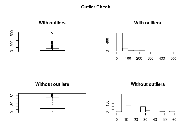
## Outliers identified: 116 nPropotion (%) of outliers: 15 nMean of the outliers: 128.29 nMean without removing outliers: 32.2 nMean if we remove outliers: 17.82 n
outlierKD(titanic_train,SibSp)
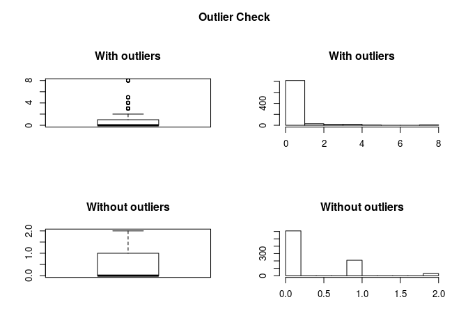
## Outliers identified: 46 nPropotion (%) of outliers: 5.4 nMean of the outliers: 4.37 nMean without removing outliers: 0.52 nMean if we remove outliers: 0.31 n
outlierKD(titanic_train,Parch)
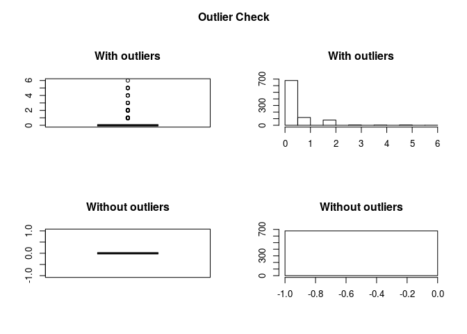
## Outliers identified: 213 nPropotion (%) of outliers: 31.4 nMean of the outliers: 1.6 nMean without removing outliers: 0.38 nMean if we remove outliers: 0 n
Checking Missing Values
checkNA <- function(x){sum(is.na(x))/length(x)*100}
sapply(titanic,checkNA)

## PassengerId    Survived      Pclass        Name         Sex         Age
##  0.00000000 31.93277311  0.00000000  0.00000000  0.00000000 20.09167303
##       SibSp       Parch      Ticket        Fare       Cabin    Embarked
##  0.00000000  0.00000000  0.00000000  0.07639419  0.00000000  0.00000000
Survived: 31.9% NA, Age:20.1% NA, Fare:.07% NA values.
Though NA values in Survived here only represent test data set so ignore Survived.
sapply(titanic_train,checkNA)

## PassengerId    Survived      Pclass        Name         Sex         Age
##     0.00000     0.00000     0.00000     0.00000     0.00000    19.86532
##       SibSp       Parch      Ticket        Fare       Cabin    Embarked
##     0.00000     0.00000     0.00000     0.00000     0.00000     0.00000
Checking Missing values which are not NA
checkMissing <- function(x){sum(x=="")/length(x)*100}
sapply(titanic,checkMissing)

## PassengerId    Survived      Pclass        Name         Sex         Age
##   0.0000000          NA   0.0000000   0.0000000   0.0000000          NA
##       SibSp       Parch      Ticket        Fare       Cabin    Embarked
##   0.0000000   0.0000000   0.0000000          NA  77.4637128   0.1527884
Cabin: 77.46%, Embarked: .15% values are empty
Missing Value Treatment
Toggle Code button to see code
#1. Age: Replacing NA values in Age with mean
#titanic[is.na(titanic$Age),6] <- mean(titanic$Age)
titanic$Age[is.na(titanic$Age)] <- round(mean(titanic$Age, na.rm = TRUE))
titanic_train$Age[is.na(titanic_train$Age)] <- round(mean(titanic_train$Age, na.rm = TRUE))

#2. Embarked: Replacing Empty Embarked with most common value 'S'
titanic_train$Embarked <- replace(titanic_train$Embarked, which(titanic_train$Embarked==""), 'S')

#3. Cabin: Not replacing with anything as Cabin values are unique
Feature Engineering
Dataset contains some attributes like Name, Age, SibSp & Parch which can be used effectively if we can extract useful information from these using regular expressions & binning.
1. Extracting Title from Name
Title <-  gsub("^.*, (.*?)\\..*$", "\\1", titanic_train$Name)
titanic_train$Title <- as.factor(Title)
table(Title)

## Title
##         Capt          Col          Don           Dr     Jonkheer
##            1            2            1            7            1
##         Lady        Major       Master         Miss         Mlle
##            1            2           40          182            2
##          Mme           Mr          Mrs           Ms          Rev
##            1          517          125            1            6
##          Sir the Countess
##            1            1
2. Extracting Family Size from SibSp & Parch
titanic_train$FamilyCount <-titanic_train$SibSp + titanic_train$Parch + 1
titanic_train$FamilySize[titanic_train$FamilyCount == 1] <- 'Single'
titanic_train$FamilySize[titanic_train$FamilyCount < 5 & titanic_train$FamilyCount >= 2] <- 'Small'
titanic_train$FamilySize[titanic_train$FamilyCount >= 5] <- 'Big'
titanic_train$FamilySize=as.factor(titanic_train$FamilySize)
table(titanic_train$FamilySize)

##
##    Big Single  Small
##     62    537    292
Data Preprocessing
Most variables in dataset are categorical, here I will update their names as per data dictionary & data types as factor for simplicity & readability. Toggle Code button to see steps.
# 1.Changing names of few categorical variables for interpretability
titanic_train$Survived <- ifelse(titanic_train$Survived==1,"Yes","No")
titanic_train$Survived <- as.factor(titanic_train$Survived)

titanic_train$Embarked <- ifelse(titanic_train$Embarked=="S","Southampton",
                              ifelse(titanic_train$Embarked=="C","Cherbourg", "Queenstown"))
titanic_train$Embarked <- as.factor(titanic_train$Embarked)

# 2.Converting categorical variables from int to factor
# i) Pclass
titanic_train$Pclass <- as.factor(titanic_train$Pclass)

# ii) SibSp
titanic_train$SibSp <- as.factor(titanic_train$SibSp)

# iii) Parch
titanic_train$Parch <- as.factor(titanic_train$Parch)
Asking questions on Titanic tragedy
Lets try to draw few insights from data using Univariate & Bivariate Analysis
Note: For queries related to passenger survival I will use train dataset as ‘Survived’ attribute is not available in test & has to be predicted using created model. So these observations will not be accurate as we don’t have complete data of passengers to analyze here.
1. What percentage of passengers survived?
temp<-subset(titanic_train,titanic_train$Survived=="Yes")
(nrow(temp)/nrow(titanic_train))*100
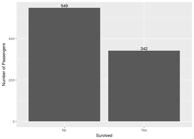 38.3% passengers survived
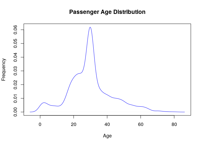
2. What was the average age of passengers?
Seems that most passengers had Age between 25-35.
summary(titanic$Age)

##    Min. 1st Qu.  Median    Mean 3rd Qu.    Max.
##    0.17   22.00   30.00   29.91   35.00   80.00

d <- density(titanic$Age)
plot(d,main="Passenger Age Distribution",xlab="Age",ylab="Frequency",col="blue")
3. What was proportion of survivors by gender?
As we know that women & children were saved first a large proportion of women survived compared to men.
ggplot(titanic_train, aes(x=Sex,fill=Survived))+ geom_bar(position = "dodge") + geom_text(stat='count',aes(label=..count..),position = position_dodge(0.9),vjust=-0.2) +
ylab("Number of Passengers")
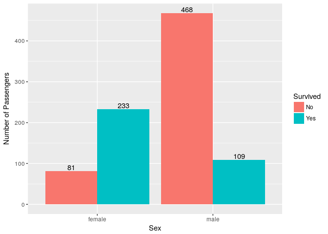
| Sex | Survived | Died | Percentage Survived |
|---|---|---|---|
| Male | 109 | 468 | 18.9% |
| Female | 233 | 81 | 74.2% |
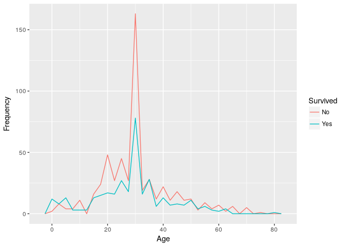
4. What was the Age distribution of Survivors & Non-Survivors?
Blue line of Survivors crosses Red line of Non-Survivors for children & elders who were saved first.
ggplot(titanic_train) + geom_freqpoly(mapping = aes(x = Age, color = Survived), binwidth = 2.5) +
ylab("Frequency")
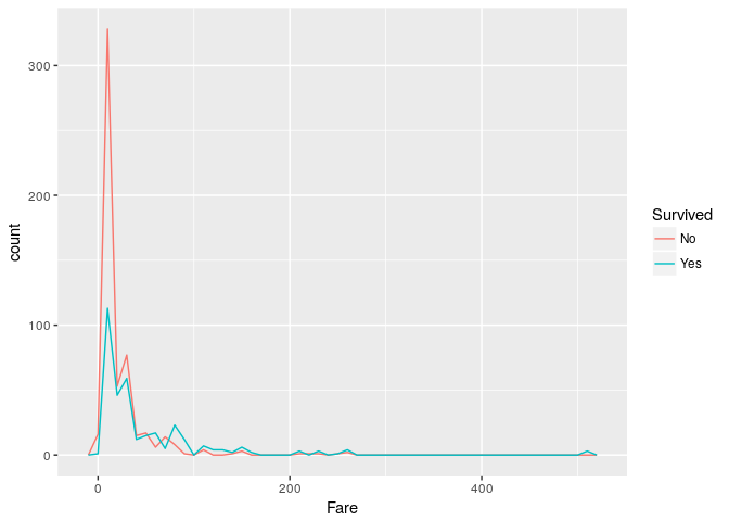
5. What was the distribution of Passenger Fare for Survivors & Non-Survivors?
Blue line crosses red line as Fare increases which might be linked to Passenger Class. Lets explore this further in next question.
ggplot(titanic_train) + geom_freqpoly(mapping = aes(x = Fare, color = Survived), binwidth = 10)
6. What was the Passenger Class of most Non-Survivors?
Most passengers from third class died, may be they didn’t get the fair chance. you can read more about this here.
ggplot(titanic_train, aes(x=Pclass,fill=Survived))+ geom_bar(position = "dodge") + geom_text(stat='count',aes(label=..count..),position = position_dodge(0.9),vjust=-0.2) +
ylab("Number of Passengers") + xlab("Passenger Class")
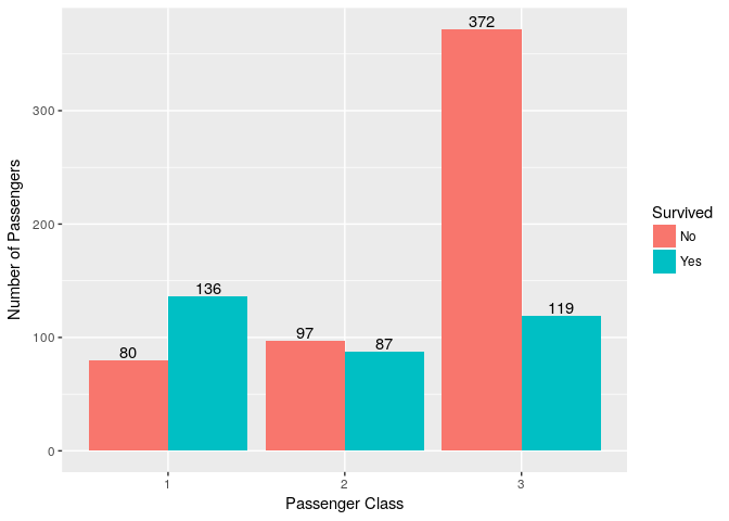
| Passenger Class | Survived | Died | Percentage Survived |
|---|---|---|---|
| Third | 119 | 372 | 24.2% |
| Second | 87 | 97 | 47.2% |
| First | 136 | 80 | 62.9% |
7. What was proportion of survivors by place of Embarkment?
A large proportion of passengers boarded from Southampton(72.4%) followed by Cherbourg(18.9%) & Queenstown(8.6%). Titanic started her maiden voyage from Southhampton, you can read more about whole route here.
ggplot(titanic_train, aes(x=Embarked,fill=Survived))+ geom_bar(position = "dodge") + geom_text(stat='count',aes(label=..count..),position = position_dodge(0.9),vjust=-0.2) +
ylab("Number of Passengers")
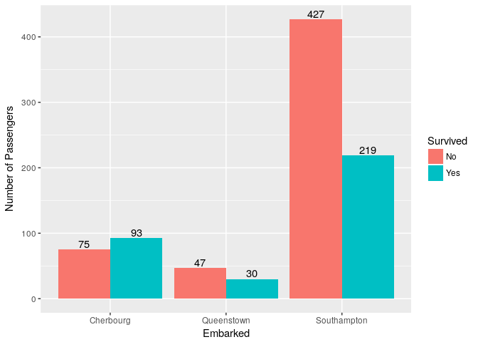
| Embarked at | Survived | Died | Percentage Survived |
|---|---|---|---|
| Southampton | 219 | 427 | 33.9% |
| Queenstown | 30 | 47 | 38.9% |
| Cherbourg | 93 | 75 | 55.3% |
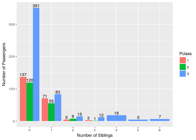
8. Were number of sibling/spouses aboard Titanic & Passenger Class related?
Mostly Class 3 Passengers had more then 3 siblings or large families compared to Class 1 & 2.
ggplot(titanic_train, aes(x=SibSp,fill=Pclass))+ geom_bar(position = "dodge") + geom_text(stat='count',aes(label=..count..),position = position_dodge(0.9),vjust=-0.2) +
ylab("Number of Passengers") + xlab("Number of Siblings")
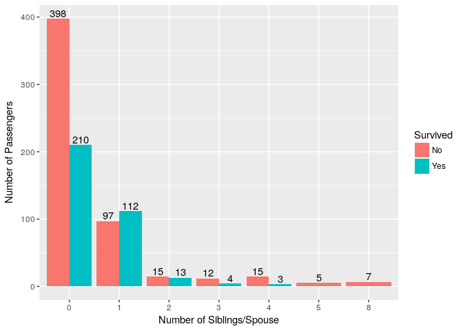
9. Was number of sibling/spouses aboard Titanic related to Survival?
ggplot(titanic_train, aes(x=SibSp,fill=Survived))+ geom_bar(position = "dodge") + geom_text(stat='count',aes(label=..count..),position = position_dodge(0.9),vjust=-0.2) +
ylab("Number of Passengers")+xlab("Number of Siblings/Spouse")
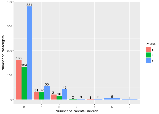
10. Does Number of parents/children aboard Titanic differ with Passenger Class?
Like SibSp Class 3 Passengers had more then 3 children or large families compared to Class 1 & 2.
ggplot(titanic_train, aes(x=Parch,fill=Pclass))+ geom_bar(position = "dodge") + geom_text(stat='count',aes(label=..count..),position = position_dodge(0.9),vjust=-0.2) +
ylab("Number of Passengers") + xlab("Number of Parents/Children")
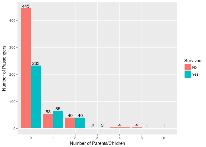
11. Was number of Parents/Children aboard Titanic related to Survival?
Although Passengers with 0 Parents/Children have smallest survival ratio this could be entirely based on probability as we have seen same pattern with SibSp, so can’t say much from this plot.
ggplot(titanic_train, aes(x=Parch,fill=Survived))+ geom_bar(position = "dodge") + geom_text(stat='count',aes(label=..count..),position = position_dodge(0.9),vjust=-0.2) +
ylab("Number of Passengers") + xlab("Number of Parents/Children")
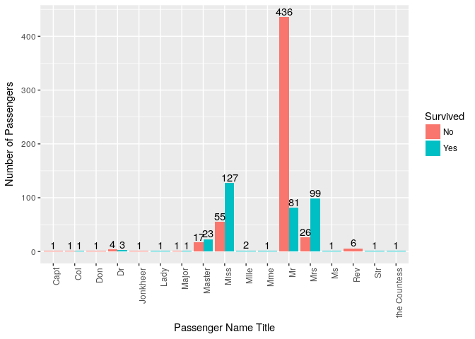
12. Was there any relation between Passenger Name Title & Survival?
As we already saw the male/female survival ratio earlier, a similar pattern exist here as male titles like ‘Mr’ have lower survival percentage compared to female title like ‘Miss’ & ‘Mrs’.
ggplot(titanic_train, aes(x=Title,fill=Survived))+ geom_bar(position = "dodge") + geom_text(stat='count',aes(label=..count..),position = position_dodge(0.9),vjust=-0.2) +
ylab("Number of Passengers") + xlab("Passenger Name Title") + theme(axis.text.x = element_text(angle = 90, hjust = 1))
13. Was there any relation between Family Size & Survival?
ggplot(titanic_train, aes(x=FamilySize,fill=Survived))+ geom_bar(position = "dodge") + geom_text(stat='count',aes(label=..count..),position = position_dodge(0.9),vjust=-0.2) +
ylab("Number of Passengers") + xlab("Family Size")
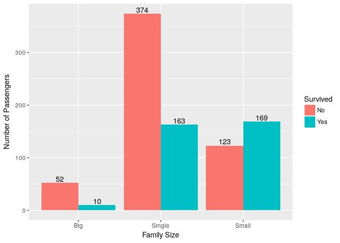
| Passenger Class | Survived | Died | Percentage Survived |
|---|---|---|---|
| Big | 10 | 52 | 16.1% |
| Small | 169 | 123 | 57.8% |
| Single | 163 | 374 | 30.3% |
We can explore many more relationships among given variables & drive new features based on maybe Cabin, Tickets etc. There are many questions which can be asked. More relevant interpretations can be drawn from complete dataset of passengers.
Thanks for reading this notebook.