Image Source
Problem Statement
To build a recommendation system using collaborative filtering, where customers will be recommended the beer that they are most likely to buy using given dataset of half million beer reviews.
Goals of Assignment:
- Choose only those beers that have at least N number of reviews, Find N using EDA.
- Clean data an find average beer & user ratings.
- Find similarity between the first 10 beers & first 10 users & plot this similarity matrix.
- Evaluate Item Based & User Based Collaborative Filtering Algorithms using ‘split’ and ‘cross-validation’ evaluation schemes.
- Recommend Top 5 beers to users “cokes”, “genog” & “giblet”.
Dataset Preview
head(beer) %>% kable("html") %>%
  kable_styling()
| beer\_beerid | review\_profilename | review\_overall |
|---|---|---|
| 48215 | stcules | 3.0 |
| 52159 | oline73 | 3.0 |
| 52159 | alpinebryant | 3.0 |
| 52159 | rawthar | 4.0 |
| 52159 | RangerClegg | 3.5 |
| 58046 | mikedrinksbeer2 | 4.5 |
Dataset contains 3 attributes Beer Id, Reviewer Name & Rating given by reviewer. Total 475984 reviews are given.
Data Structure
str(beer)

## 'data.frame':    475984 obs. of  3 variables:
##  $ beer_beerid       : int  48215 52159 52159 52159 52159 58046 58046 58046 58046 58046 ...
##  $ review_profilename: Factor w/ 22498 levels "","0110x011",..: 19293 15474 675 16851 16798 13843 5629 2680 1473 15351 ...
##  $ review_overall    : num  3 3 3 4 3.5 4.5 4 4.5 4.5 4 ...
Data Summary
summary(beer)

##   beer_beerid         review_profilename review_overall
##  Min.   :    3   northyorksammy:  1846   Min.   :0.000
##  1st Qu.: 1716   mikesgroove   :  1379   1st Qu.:3.500
##  Median :13892   BuckeyeNation :  1338   Median :4.000
##  Mean   :21661   Thorpe429     :  1072   Mean   :3.815
##  3rd Qu.:39397   ChainGangGuy  :  1046   3rd Qu.:4.500
##  Max.   :77317   NeroFiddled   :  1031   Max.   :5.000
##                  (Other)       :468272
Missing Values
Total 100 reviews have empty review_profilename.
nrow(beer[(is.na(beer$review_profilename) | beer$review_profilename==""), ])

## [1] 100
Updating beer datset removing empty review_profilename.
beer<-beer[!(beer$review_profilename==""), ]
Checking Duplicates
Checking for duplicates where both item and user are duplicated or same user gave multiple ratings to same beer.
beer[!(duplicated(beer[c("beer_beerid","review_profilename")]) | duplicated(beer[c("beer_beerid","review_profilename")], fromLast = TRUE)), ] %>% nrow()

## [1] 473055

beer %>% distinct(beer_beerid,review_profilename,.keep_all = TRUE) %>% nrow()

## [1] 474462
474462 distinct reviews
Removing duplicates having both beer & user duplicated, this will ensure that no 2 reviews from single user to same beer are counted & cumulate.
beer<-distinct(beer,beer_beerid,review_profilename,.keep_all = TRUE)
I. Data Preparation
1. Choose only those beers that have at least N number of reviews
Lets find all distinct beers & total reviews they received
beer_reviews_count <- beer %>% group_by(beer_beerid) %>% summarise(total_beer_reviews=n())
dim(beer_reviews_count)

## [1] 40304     2
Total 40308 distinct beers.
Lets sort these beers by reviews
 beer_reviews_count[with(beer_reviews_count, order(total_beer_reviews,decreasing = TRUE)), ]

## # A tibble: 40,304 x 2
##    beer_beerid total_beer_reviews
##          <int>              <int>
##  1        2093                977
##  2         412                966
##  3        1904                902
##  4        1093                840
##  5          92                812
##  6        4083                798
##  7         276                788
##  8        7971                778
##  9          88                755
## 10        1013                750
## # ... with 40,294 more rows

summary(beer_reviews_count)

##   beer_beerid    total_beer_reviews
##  Min.   :    3   Min.   :  1.00
##  1st Qu.:16880   1st Qu.:  1.00
##  Median :37366   Median :  2.00
##  Mean   :36973   Mean   : 11.77
##  3rd Qu.:56234   3rd Qu.:  5.00
##  Max.   :77317   Max.   :977.00
Beers have reviews count in range of 1 to 987, beer 2093 have highest number of reviews(987).
Lets also count number of distinct users
beer %>% group_by(review_profilename) %>% summarise(total_user_reviews=n()) %>% nrow()

## [1] 22497
22497 distinct users
Lets now check which user have reviewed maximum beers
beer %>% group_by(review_profilename) %>% summarise(user_review_count=n()) %>% top_n(1)

## Selecting by user_review_count

## # A tibble: 1 x 2
##   review_profilename user_review_count
##               <fctr>             <int>
## 1     northyorksammy              1842
user: northyorksammy have given max reviews:1842
To find an ideal value of N its important that we choose beers hacing large enough number of reviews to avoid cold start problem.
So Lets further analyze beers by number of reviews each one have received. lets start with all beers with single review.
qplot(beer_reviews_count$total_beer_reviews, geom = "histogram",xlab="Total Reviews")

## `stat_bin()` using `bins = 30`. Pick better value with `binwidth`.
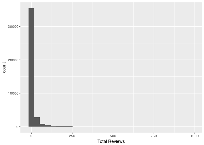
beer_reviews_count %>% subset(total_beer_reviews==1) %>% dim()

## [1] 18080     2
#So 18080 or 44.7% beers have only 1 review, lets group by total reviews & find count for each.
Lets create separate dataframe with frequency of count of reviews
review_frequency<-beer_reviews_count %>% group_by(total_beer_reviews) %>% summarise(review_occurance=n())

head(review_frequency,25)

## # A tibble: 25 x 2
##    total_beer_reviews review_occurance
##                 <int>            <int>
##  1                  1            18080
##  2                  2             6183
##  3                  3             3079
##  4                  4             1895
##  5                  5             1350
##  6                  6              959
##  7                  7              785
##  8                  8              556
##  9                  9              478
## 10                 10              401
## # ... with 15 more rows
It seems that most beers get very few reviews. Infact very few beers have large enough number of reviews required for building recommendation system based on collaborative filtering.
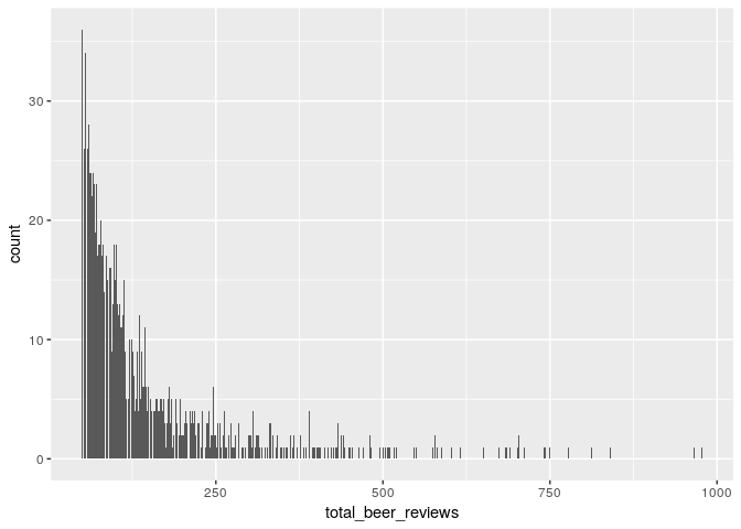
Filtering by beers having at least 50 reviews & users having reviewed at least 30 beers as there are more distinct beers(40308)
beer_reviews_count_subset<-subset(beer_reviews_count,beer_reviews_count$total_beer_reviews>=50)
Now we are left with a dataset of these distinct beer ids each having more than 50 reviews each.
Lets check beer review frequency now
ggplot(beer_reviews_count_subset,aes(x=total_beer_reviews)) + geom_bar()
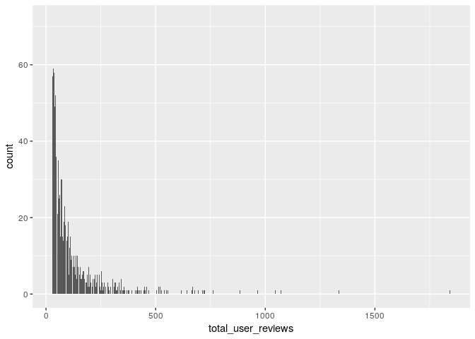
Lets also filter beer dataset based on users who have atleast reviewd 30 beers each
user_reviews_count<- beer %>% group_by(review_profilename) %>% summarise(total_user_reviews=n())
user_reviews_count_subset<-subset(user_reviews_count,user_reviews_count$total_user_reviews>=30)
ggplot(user_reviews_count_subset,aes(x=total_user_reviews)) + geom_bar()
Now lets filter original data by these beer and user ids
important_beers<-merge(beer,beer_reviews_count_subset,by.x="beer_beerid",by.y="beer_beerid")
important_beers<-merge(important_beers,user_reviews_count_subset,by.x="review_profilename",by.y="review_profilename")

summary(important_beers)

##       review_profilename  beer_beerid    review_overall total_beer_reviews
##  BuckeyeNation :   518   Min.   :    5   Min.   :1.00   Min.   : 50.0
##  mikesgroove   :   505   1st Qu.: 1089   1st Qu.:3.50   1st Qu.: 97.0
##  BEERchitect   :   460   Median : 4161   Median :4.00   Median :171.0
##  northyorksammy:   455   Mean   :15774   Mean   :3.87   Mean   :233.8
##  WesWes        :   455   3rd Qu.:29619   3rd Qu.:4.50   3rd Qu.:314.0
##  TheManiacalOne:   440   Max.   :75086   Max.   :5.00   Max.   :977.0
##  (Other)       :227255
##  total_user_reviews
##  Min.   :  30.0
##  1st Qu.:  78.0
##  Median : 155.0
##  Mean   : 233.1
##  3rd Qu.: 299.0
##  Max.   :1842.0
##
This beer subset have substantial ratings by both users & beers.
2. Convert this data frame to a “realratingMatrix” before you build your collaborative filtering models
beers_rrmatrix <- as(important_beers[,c(1,2,3)], "realRatingMatrix")
class(beers_rrmatrix)

## [1] "realRatingMatrix"
## attr(,"package")
## [1] "recommenderlab"
Checking realRatingMatrix
Few reviews by each user
head(rowCounts(beers_rrmatrix))

##  0110x011  05Harley 100floods  1759Girl  1fastz28  32hoss32
##        30        30        29        40        96        26
Few reviews given to beers
head(colCounts(beers_rrmatrix))

##   5   6   7  10  14  15
##  92 190 147 181  51  45
Average ratings by few users
head(rowMeans(beers_rrmatrix))

##  0110x011  05Harley 100floods  1759Girl  1fastz28  32hoss32
##  4.333333  4.116667  4.155172  3.725000  3.875000  3.788462
Converting the matrix to a dataframe
beers_df <- as(beers_rrmatrix, "data.frame")
str(beers_df)

## 'data.frame':    230088 obs. of  3 variables:
##  $ user  : Factor w/ 3176 levels "0110x011","05Harley",..: 1 1 1 1 1 1 1 1 1 1 ...
##  $ item  : Factor w/ 2064 levels "10","100","1002",..: 2039 47 256 263 1165 1750 1925 1955 2007 24 ...
##  $ rating: num  4 4 4.5 4.5 4.5 4 5 4 5 4 ...

summary(beers_df)

##              user             item            rating
##  BuckeyeNation :   518   2093   :   600   Min.   :1.00
##  mikesgroove   :   505   412    :   589   1st Qu.:3.50
##  BEERchitect   :   460   1904   :   574   Median :4.00
##  northyorksammy:   455   1093   :   552   Mean   :3.87
##  WesWes        :   455   4083   :   525   3rd Qu.:4.50
##  TheManiacalOne:   440   1013   :   515   Max.   :5.00
##  (Other)       :227255   (Other):226733
II. Data Exploration:
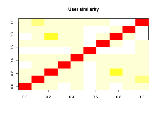
1. Determine how similar the first ten users are with each other and visualize it
How similar are the first ten users are with each other
similar_users <- similarity(beers_rrmatrix[1:10,],method = "cosine",which = "users")
Users Similarity matrix
kable(as.matrix(similar_users))
| 0110x011 | 05Harley | 100floods | 1759Girl | 1fastz28 | 32hoss32 | 3Vandoo | 4000qtrap | 4DAloveofSTOUT | 51mmz0rz | |
|---|---|---|---|---|---|---|---|---|---|---|
| 0110x011 | 0.0000000 | 1.0000000 | 1.0000000 | NA | 0.9986178 | NA | 1.0000000 | NA | 1.0000000 | 1.0000000 |
| 05Harley | 1.0000000 | 0.0000000 | 0.9982744 | 1.0000000 | 0.9801961 | NA | 1.0000000 | 1.0000000 | 0.9986898 | 0.8944272 |
| 100floods | 1.0000000 | 0.9982744 | 0.0000000 | 1.0000000 | 0.9986226 | NA | 1.0000000 | 0.8106792 | 0.9982744 | 0.9474403 |
| 1759Girl | NA | 1.0000000 | 1.0000000 | 0.0000000 | 0.9975295 | NA | 0.9970831 | 1.0000000 | 0.9970545 | 0.9727176 |
| 1fastz28 | 0.9986178 | 0.9801961 | 0.9986226 | 0.9975295 | 0.0000000 | 0.9959184 | 0.9938707 | 0.9977852 | 1.0000000 | 0.9626219 |
| 32hoss32 | NA | NA | NA | NA | 0.9959184 | 0.0000000 | NA | NA | NA | 1.0000000 |
| 3Vandoo | 1.0000000 | 1.0000000 | 1.0000000 | 0.9970831 | 0.9938707 | NA | 0.0000000 | 0.9998377 | NA | 1.0000000 |
| 4000qtrap | NA | 1.0000000 | 0.8106792 | 1.0000000 | 0.9977852 | NA | 0.9998377 | 0.0000000 | 0.9969278 | NA |
| 4DAloveofSTOUT | 1.0000000 | 0.9986898 | 0.9982744 | 0.9970545 | 1.0000000 | NA | NA | 0.9969278 | 0.0000000 | NA |
| 51mmz0rz | 1.0000000 | 0.8944272 | 0.9474403 | 0.9727176 | 0.9626219 | 1.0000000 | 1.0000000 | NA | NA | 0.0000000 |
Visualize similarity matrix
image(as.matrix(similar_users), main = "User similarity")
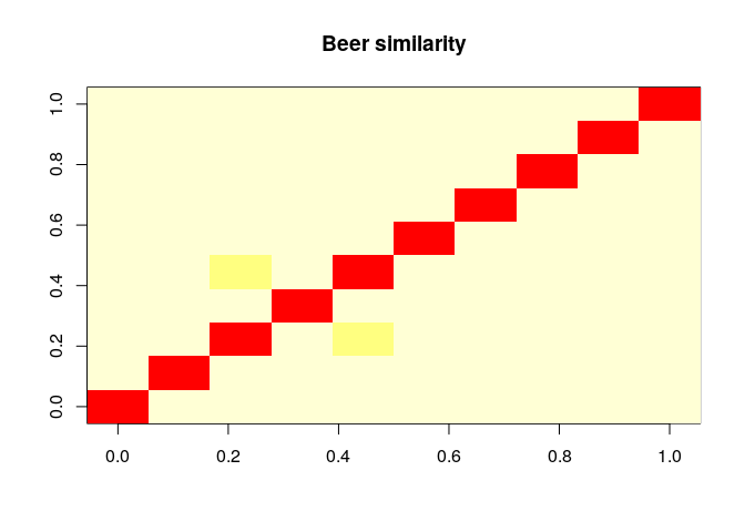
2. Compute and visualize the similarity between the first 10 beers
How similar are the first ten beers are with each other
similar_beers <- similarity(beers_rrmatrix[,1:10],method = "cosine",which = "items")
Items(Beers) Similarity matrix
kable(as.matrix(similar_beers))
| 5 | 6 | 7 | 10 | 14 | 15 | 17 | 19 | 30 | 31 | |
|---|---|---|---|---|---|---|---|---|---|---|
| 5 | 0.0000000 | 0.9726805 | 0.9783900 | 0.9312075 | 0.9933630 | 0.9815302 | 0.9519402 | 0.9607689 | 0.9634705 | 0.9710609 |
| 6 | 0.9726805 | 0.0000000 | 0.9469754 | 0.9877854 | 0.9542911 | 0.9865850 | 0.9633901 | 0.9653313 | 0.9829763 | 0.9822110 |
| 7 | 0.9783900 | 0.9469754 | 0.0000000 | 0.9491052 | 0.8717101 | 0.9674071 | 0.9561002 | 0.9323216 | 0.9459190 | 0.9260756 |
| 10 | 0.9312075 | 0.9877854 | 0.9491052 | 0.0000000 | 0.9615401 | 0.9764387 | 0.9742800 | 0.9852062 | 0.9917181 | 0.9854066 |
| 14 | 0.9933630 | 0.9542911 | 0.8717101 | 0.9615401 | 0.0000000 | 0.9934646 | 0.9601002 | 0.9905018 | 0.9894903 | 0.9711294 |
| 15 | 0.9815302 | 0.9865850 | 0.9674071 | 0.9764387 | 0.9934646 | 0.0000000 | 0.9804572 | 0.9835829 | 0.9948577 | 0.9951374 |
| 17 | 0.9519402 | 0.9633901 | 0.9561002 | 0.9742800 | 0.9601002 | 0.9804572 | 0.0000000 | 0.9768746 | 0.9744582 | 0.9640672 |
| 19 | 0.9607689 | 0.9653313 | 0.9323216 | 0.9852062 | 0.9905018 | 0.9835829 | 0.9768746 | 0.0000000 | 0.9893860 | 0.9827195 |
| 30 | 0.9634705 | 0.9829763 | 0.9459190 | 0.9917181 | 0.9894903 | 0.9948577 | 0.9744582 | 0.9893860 | 0.0000000 | 0.9884008 |
| 31 | 0.9710609 | 0.9822110 | 0.9260756 | 0.9854066 | 0.9711294 | 0.9951374 | 0.9640672 | 0.9827195 | 0.9884008 | 0.0000000 |
Visualize similarity matrix
image(as.matrix(similar_beers), main = "Beer similarity")
3. What are the unique values of ratings?
beers_df %>% group_by(rating) %>% summarise(rating_frequency=n()) %>% nrow()

## [1] 9
So 9 distinct ratings, lets check frequency of each rating.
beers_df %>% group_by(rating) %>% summarise(rating_frequency=n())

## # A tibble: 9 x 2
##   rating rating_frequency
##    <dbl>            <int>
## 1    1.0             1120
## 2    1.5             1343
## 3    2.0             4474
## 4    2.5             7012
## 5    3.0            21189
## 6    3.5            42543
## 7    4.0            88240
## 8    4.5            51086
## 9    5.0            13081
So rating 4.0 & 4.5 are most common, 1.0 & 1.5 are least common.
4. Visualize the rating values and notice:
(i) The average beer ratings
avg_beer_ratings<-beers_df %>% group_by(item) %>% summarise(average_rating=mean(rating))

colors <- c(rep("red",2), rep("blue",2), rep("green",1))
ggplot(avg_beer_ratings,aes(x=average_rating)) + geom_histogram() + labs(x="Average Rating", y="Number of Beers") + scale_x_discrete(limits=1:5)

## `stat_bin()` using `bins = 30`. Pick better value with `binwidth`.
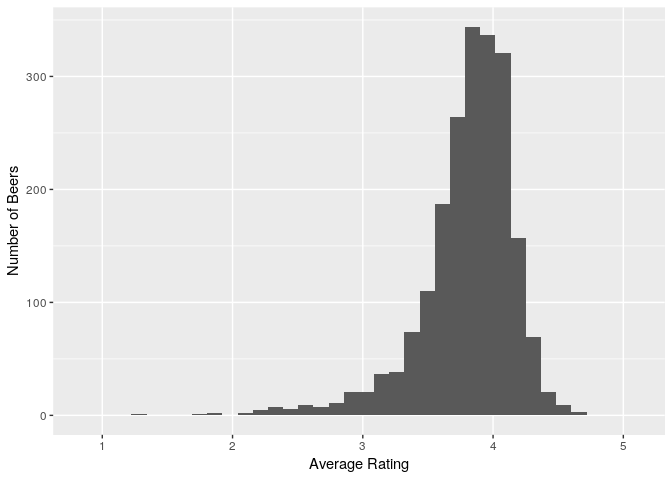
summary(avg_beer_ratings$average_rating)

##    Min. 1st Qu.  Median    Mean 3rd Qu.    Max.
##   1.258   3.656   3.870   3.806   4.043   4.636
So average beer ratings(Mean)=3.898 & Median=3.955, almost normal, slightly left skewed.
Also checking on original full dataset of beers
avg_beer_ratings_all<-beer %>% group_by(beer_beerid) %>% summarise(average_rating=mean(review_overall))
ggplot(avg_beer_ratings_all,aes(x=average_rating)) + geom_histogram() + labs(x="Average Rating", y="# of Beers")

## `stat_bin()` using `bins = 30`. Pick better value with `binwidth`.
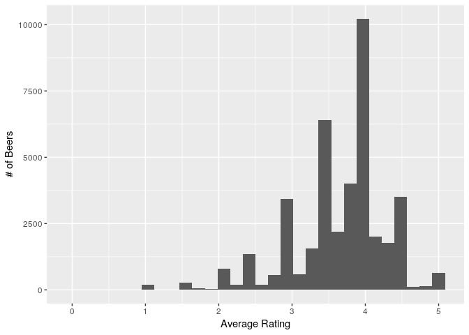
summary(avg_beer_ratings_all$average_rating)

##    Min. 1st Qu.  Median    Mean 3rd Qu.    Max.
##   0.000   3.500   3.800   3.671   4.000   5.000
So average beer ratings(Mean)=3.8 & Median=4, uneven distribution.
(ii) The average user ratings
avg_user_ratings<-beers_df %>% group_by(user) %>% summarise(average_rating=mean(rating))
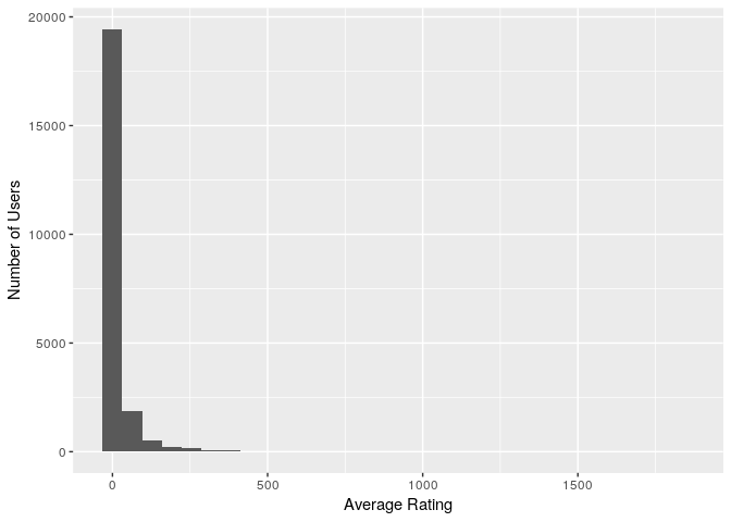
ggplot(avg_user_ratings,aes(x=average_rating)) + geom_histogram() + labs(x="Average Rating", y="Number of Users")
## `stat_bin()` using `bins = 30`. Pick better value with `binwidth`.
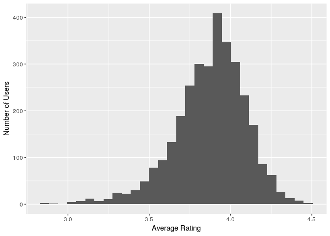
summary(avg_user_ratings$average_rating)

##    Min. 1st Qu.  Median    Mean 3rd Qu.    Max.
##   2.833   3.750   3.901   3.875   4.023   4.457
So average beer ratings(Mean)=3.991 & Median=4, slightly left skewed & uneven distribution.
(iii) The average number of ratings given to the beers
avg_beer_reviews<-important_beers %>% group_by(beer_beerid) %>% summarise(average_reviews=mean(total_beer_reviews))
ggplot(avg_beer_reviews,aes(x=average_reviews)) + geom_histogram() + labs(x="Average Rating", y="Number of Beers")

## `stat_bin()` using `bins = 30`. Pick better value with `binwidth`.
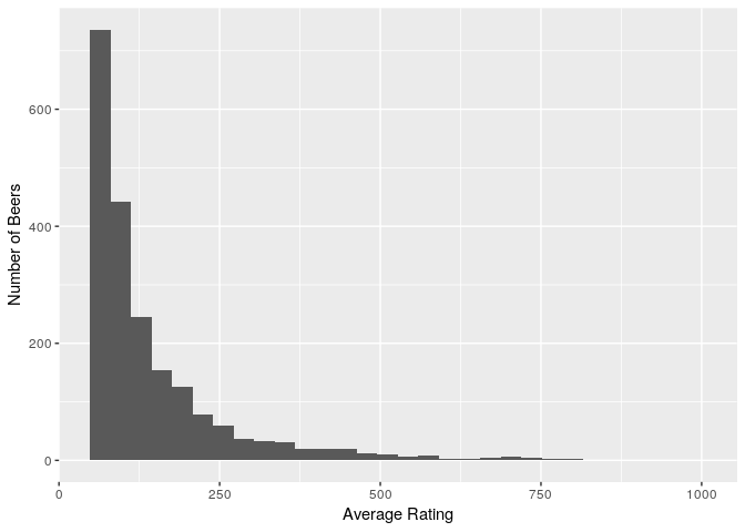
summary(avg_beer_reviews$average_reviews)

##    Min. 1st Qu.  Median    Mean 3rd Qu.    Max.
##    50.0    68.0    99.0   143.4   168.0   977.0
So on average each beer gets ~143 reviews from chosen subset.
Also checking on original full dataset of beers
avg_user_ratings_all<-beer_reviews_count %>% group_by(beer_beerid) %>% summarise(average_rating=mean(total_beer_reviews))
ggplot(avg_user_ratings_all,aes(x=average_rating)) + geom_histogram() + labs(x="Average Rating", y="Number of Users")

## `stat_bin()` using `bins = 30`. Pick better value with `binwidth`.
summary(avg_user_ratings_all$average_rating)

##    Min. 1st Qu.  Median    Mean 3rd Qu.    Max.
##    1.00    1.00    2.00   11.77    5.00  977.00
So on average each beer gets ~12 reviews.
(iv) The average number of ratings given by the users
avg_user_reviews<-important_beers %>% group_by(review_profilename) %>% summarise(average_reviews=mean(total_user_reviews))
ggplot(avg_user_reviews,aes(x=average_reviews)) + geom_histogram()

## `stat_bin()` using `bins = 30`. Pick better value with `binwidth`.
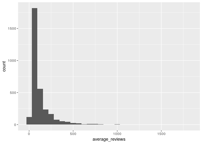
summary(avg_user_reviews$average_reviews)

##    Min. 1st Qu.  Median    Mean 3rd Qu.    Max.
##    30.0    44.0    72.0   120.9   137.2  1842.0
So on average each user gives ~101 reviews, but this distribution is very skewed.
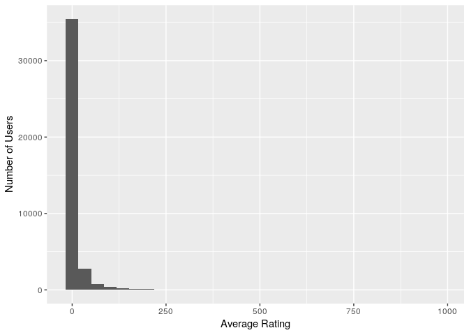
Also checking on original full dataset of beers
avg_user_ratings_all<-user_reviews_count %>% group_by(review_profilename) %>% summarise(average_rating=mean(total_user_reviews))
ggplot(avg_user_ratings_all,aes(x=average_rating)) + geom_histogram() + labs(x="Average Rating", y="Number of Users")

## `stat_bin()` using `bins = 30`. Pick better value with `binwidth`.
summary(avg_user_ratings_all$average_rating)

##    Min. 1st Qu.  Median    Mean 3rd Qu.    Max.
##    1.00    1.00    3.00   21.09   11.00 1842.00
So on average each user gives 21 reviews, but this distribution is very skewed.
Also Visualizing ratings with real rating matrix of beers
qplot(getRatings(beers_rrmatrix), binwidth = 1, main = "Histogram of ratings", xlab = "Rating")
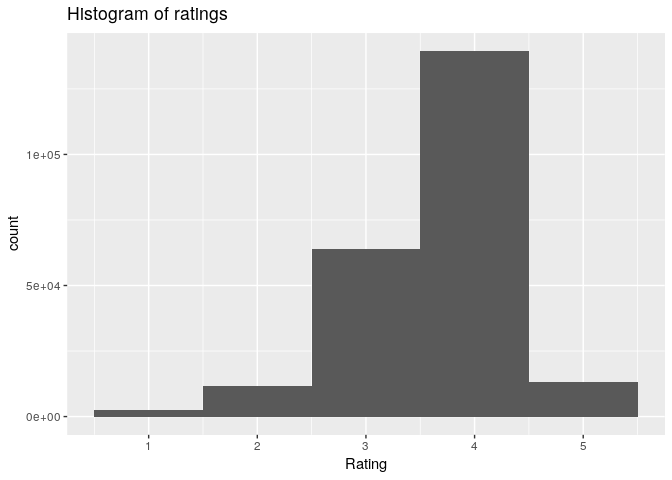
summary(getRatings(beers_rrmatrix)) #slightly right skewed

##    Min. 1st Qu.  Median    Mean 3rd Qu.    Max.
##    1.00    3.50    4.00    3.87    4.50    5.00

qplot(getRatings(normalize(beers_rrmatrix, method = "Z-score")),main = "Histogram of normalized ratings", xlab = "Rating")

## `stat_bin()` using `bins = 30`. Pick better value with `binwidth`.
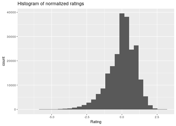
summary(getRatings(normalize(beers_rrmatrix, method = "Z-score"))) # seems better

##    Min. 1st Qu.  Median    Mean 3rd Qu.    Max.
## -6.5750 -0.5318  0.1276  0.0000  0.6984  3.2030

qplot(rowCounts(beers_rrmatrix), binwidth = 10,
      main = "Beers Rated on average", xlab = "# of users", ylab = "# of beers rated")
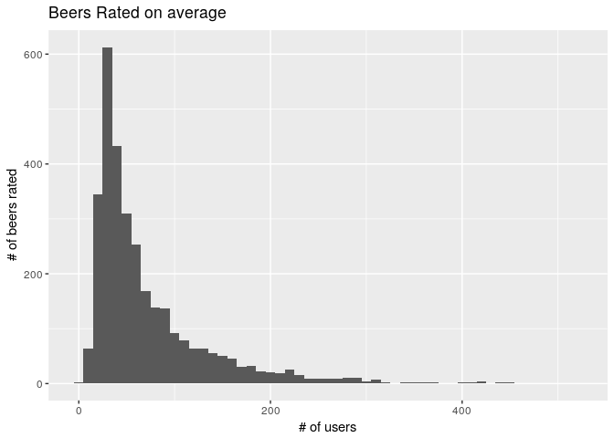
Most users rate less number of beers, very few users have rated more beers
III. Recommendation Models:
1. Divide your data into training and testing datasets, Experiment with ‘split’ and ‘cross-validation’ evaluation schemes
- Scheme1 with train/test(90/10) using split without cross validation & goodRating as 4
scheme1 <- evaluationScheme(beers_rrmatrix, method = "split", train = .75,k = 1, given = -1, goodRating = 4)
scheme1

## Evaluation scheme using all-but-1 items
## Method: 'split' with 1 run(s).
## Training set proportion: 0.750
## Good ratings: >=4.000000
## Data set: 3176 x 2064 rating matrix of class 'realRatingMatrix' with 230088 ratings.
- Scheme2 using cross-validation without cross validation(5 folds) & goodRating as 4
scheme2 <- evaluationScheme(beers_rrmatrix, method = "cross-validation",k = 5, given = -1, goodRating = 4)
scheme2

## Evaluation scheme using all-but-1 items
## Method: 'cross-validation' with 5 run(s).
## Good ratings: >=4.000000
## Data set: 3176 x 2064 rating matrix of class 'realRatingMatrix' with 230088 ratings.
2. Building IBCF and UBCF models with below hyperparameters
algorithms <- list(
  "user-based CF" = list(name="UBCF", param=list(normalize = "Z-score",
                                                 method="Cosine",
                                                 nn=30)),
  "item-based CF" = list(name="IBCF", param=list(normalize = "Z-score")))
Evaluating algorithms & predicting next n beers
results1 <- evaluate(scheme1, algorithms, n=c(1, 3, 5, 10, 15, 20))

## UBCF run fold/sample [model time/prediction time]
##   1  [0.06sec/10.44sec]
## IBCF run fold/sample [model time/prediction time]
##   1  [21.42sec/0.74sec]

class(results1)

## [1] "evaluationResultList"
## attr(,"package")
## [1] "recommenderlab"

results2 <- evaluate(scheme2, algorithms, n=c(1, 3, 5, 10, 15, 20))

## UBCF run fold/sample [model time/prediction time]
##   1  [0.052sec/7.712sec]
##   2  [0.048sec/7.492sec]
##   3  [0.052sec/7.88sec]
##   4  [0.052sec/7.668sec]
##   5  [0.056sec/7.832sec]
## IBCF run fold/sample [model time/prediction time]
##   1  [25.072sec/0.504sec]
##   2  [24.016sec/0.476sec]
##   3  [23.268sec/0.492sec]
##   4  [37.936sec/0.488sec]
##   5  [36.488sec/0.48sec]

class(results2)

## [1] "evaluationResultList"
## attr(,"package")
## [1] "recommenderlab"
Note: Evaluate on scheme1 & scheme2 takes around 10 mins on my system
3. Compare the performance of the two models and suggest the one that should be deployed
Drawing ROC curve
plot(results1, annotate = 1:4, legend="topleft")
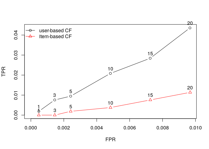
plot(results2, annotate = 1:4, legend="topleft")
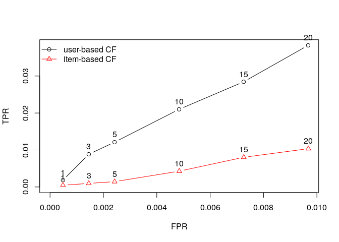
So UBCF seems to get better then IBCF especially with higher values of n.
4. Give the names of the top 5 beers that you would recommend to the users “cokes”, “genog” & “giblet”
Making Recommendations using UBCF
r <- Recommender(beers_rrmatrix, method = "UBCF")
r

## Recommender of type 'UBCF' for 'realRatingMatrix'
## learned using 3176 users.
recom_cokes <- predict(r, beers_rrmatrix['cokes'], n=5)
as(recom_cokes, "list")

## $cokes
## [1] "7971" "645"  "1346" "582"  "2041"
recom_genog <- predict(r, beers_rrmatrix['genog'], n=5)
as(recom_genog, "list")

## $genog
## [1] "57908" "1160"  "1093"  "1161"  "1445"
recom_giblet <- predict(r, beers_rrmatrix['giblet'], n=5)
as(recom_giblet, "list")

## $giblet
## [1] "19960" "4083"  "582"   "11757" "2041"