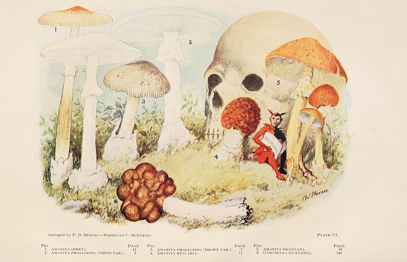
Image Source
About dataset:
I took this dataset from kaggle(https://www.kaggle.com/mig555/mushroom-classification/data) though it was originally contributed to the UCI Machine Learning repository nearly 30 years ago.
This dataset includes descriptions of hypothetical samples corresponding to 23 species of gilled mushrooms in the Agaricus and Lepiota Family Mushroom drawn from The Audubon Society Field Guide to North American Mushrooms (1981). Each species is identified as definitely edible, definitely poisonous, or of unknown edibility and not recommended. This latter class was combined with the poisonous one. The Guide clearly states that there is no simple rule for determining the edibility of a mushroom; no rule like “leaflets three, let it be’’ for Poisonous Oak and Ivy.
Problem & Approach:
To develop a binary classifier to predict which mushroom is poisonous & which is edible. I will build a Naive Bayes classifier for prediction after basic EDA of data. Later I will also test Decision Tree & Random Forest models on this dataset.
Lets check data structure
str(mushroom)

## 'data.frame':    8124 obs. of  23 variables:
##  $ class                   : Factor w/ 2 levels "e","p": 2 1 1 2 1 1 1 1 2 1 ...
##  $ cap.shape               : Factor w/ 6 levels "b","c","f","k",..: 6 6 1 6 6 6 1 1 6 1 ...
##  $ cap.surface             : Factor w/ 4 levels "f","g","s","y": 3 3 3 4 3 4 3 4 4 3 ...
##  $ cap.color               : Factor w/ 10 levels "b","c","e","g",..: 5 10 9 9 4 10 9 9 9 10 ...
##  $ bruises                 : Factor w/ 2 levels "f","t": 2 2 2 2 1 2 2 2 2 2 ...
##  $ odor                    : Factor w/ 9 levels "a","c","f","l",..: 7 1 4 7 6 1 1 4 7 1 ...
##  $ gill.attachment         : Factor w/ 2 levels "a","f": 2 2 2 2 2 2 2 2 2 2 ...
##  $ gill.spacing            : Factor w/ 2 levels "c","w": 1 1 1 1 2 1 1 1 1 1 ...
##  $ gill.size               : Factor w/ 2 levels "b","n": 2 1 1 2 1 1 1 1 2 1 ...
##  $ gill.color              : Factor w/ 12 levels "b","e","g","h",..: 5 5 6 6 5 6 3 6 8 3 ...
##  $ stalk.shape             : Factor w/ 2 levels "e","t": 1 1 1 1 2 1 1 1 1 1 ...
##  $ stalk.root              : Factor w/ 5 levels "?","b","c","e",..: 4 3 3 4 4 3 3 3 4 3 ...
##  $ stalk.surface.above.ring: Factor w/ 4 levels "f","k","s","y": 3 3 3 3 3 3 3 3 3 3 ...
##  $ stalk.surface.below.ring: Factor w/ 4 levels "f","k","s","y": 3 3 3 3 3 3 3 3 3 3 ...
##  $ stalk.color.above.ring  : Factor w/ 9 levels "b","c","e","g",..: 8 8 8 8 8 8 8 8 8 8 ...
##  $ stalk.color.below.ring  : Factor w/ 9 levels "b","c","e","g",..: 8 8 8 8 8 8 8 8 8 8 ...
##  $ veil.type               : Factor w/ 1 level "p": 1 1 1 1 1 1 1 1 1 1 ...
##  $ veil.color              : Factor w/ 4 levels "n","o","w","y": 3 3 3 3 3 3 3 3 3 3 ...
##  $ ring.number             : Factor w/ 3 levels "n","o","t": 2 2 2 2 2 2 2 2 2 2 ...
##  $ ring.type               : Factor w/ 5 levels "e","f","l","n",..: 5 5 5 5 1 5 5 5 5 5 ...
##  $ spore.print.color       : Factor w/ 9 levels "b","h","k","n",..: 3 4 4 3 4 3 3 4 3 3 ...
##  $ population              : Factor w/ 6 levels "a","c","n","s",..: 4 3 3 4 1 3 3 4 5 4 ...
##  $ habitat                 : Factor w/ 7 levels "d","g","l","m",..: 6 2 4 6 2 2 4 4 2 4 ...
Renaming all entities
As you might have noticed all data entities are named by initials only. Lets convert these to proper names for clarity & also convert all attributes to factors as all attributes are categorical here.
colnames(mushroom) <- c("Edibility", "CapShape", "CapSurface",
                        "CapColor", "Bruises", "Odor",
                        "GillAttachment", "GillSpacing", "GillSize",
                        "GillColor", "StalkShape", "StalkRoot",
                        "StalkSurfaceAboveRing", "StalkSurfaceBelowRing", "StalkColorAboveRing",
                        "StalkColorBelowRing", "VeilType", "VeilColor",
                        "RingNumber", "RingType", "SporePrintColor",
                        "Population", "Habitat")

mushroom <- mushroom %>% map_df(function(.x) as.factor(.x))

levels(mushroom$Edibility) <- c("edible", "poisonous")
levels(mushroom$CapShape) <- c("bell", "conical", "flat", "knobbed", "sunken", "convex")
levels(mushroom$CapColor) <- c("buff", "cinnamon", "red", "gray", "brown", "pink",
                                "green", "purple", "white", "yellow")
levels(mushroom$CapSurface) <- c("fibrous", "grooves", "scaly", "smooth")
levels(mushroom$Bruises) <- c("no", "yes")
levels(mushroom$Odor) <- c("almond", "creosote", "foul", "anise", "musty", "none", "pungent", "spicy", "fishy")
levels(mushroom$GillAttachment) <- c("attached", "free")
levels(mushroom$GillSpacing) <- c("close", "crowded")
levels(mushroom$GillSize) <- c("broad", "narrow")
levels(mushroom$GillColor) <- c("buff", "red", "gray", "chocolate", "black", "brown", "orange",
                                 "pink", "green", "purple", "white", "yellow")
levels(mushroom$StalkShape) <- c("enlarging", "tapering")
levels(mushroom$StalkRoot) <- c("missing", "bulbous", "club", "equal", "rooted")
levels(mushroom$StalkSurfaceAboveRing) <- c("fibrous", "silky", "smooth", "scaly")
levels(mushroom$StalkSurfaceBelowRing) <- c("fibrous", "silky", "smooth", "scaly")
levels(mushroom$StalkColorAboveRing) <- c("buff", "cinnamon", "red", "gray", "brown", "pink",
                                "green", "purple", "white", "yellow")
levels(mushroom$StalkColorBelowRing) <- c("buff", "cinnamon", "red", "gray", "brown", "pink",
                                "green", "purple", "white", "yellow")
levels(mushroom$VeilType) <- "partial"
levels(mushroom$VeilColor) <- c("brown", "orange", "white", "yellow")
levels(mushroom$RingNumber) <- c("none", "one", "two")
levels(mushroom$RingType) <- c("evanescent", "flaring", "large", "none", "pendant")
levels(mushroom$SporePrintColor) <- c("buff", "chocolate", "black", "brown", "orange",
                                        "green", "purple", "white", "yellow")
levels(mushroom$Population) <- c("abundant", "clustered", "numerous", "scattered", "several", "solitary")
levels(mushroom$Habitat) <- c("wood", "grasses", "leaves", "meadows", "paths", "urban", "waste")
Lets check few records from dataset now
head(mushroom) %>% kable("html") %>%
  kable_styling()
| Edibility | CapShape | CapSurface | CapColor | Bruises | Odor | GillAttachment | GillSpacing | GillSize | GillColor | StalkShape | StalkRoot | StalkSurfaceAboveRing | StalkSurfaceBelowRing | StalkColorAboveRing | StalkColorBelowRing | VeilType | VeilColor | RingNumber | RingType | SporePrintColor | Population | Habitat |
|---|---|---|---|---|---|---|---|---|---|---|---|---|---|---|---|---|---|---|---|---|---|---|
| poisonous | convex | scaly | brown | yes | pungent | free | close | narrow | black | enlarging | equal | smooth | smooth | purple | purple | partial | white | one | pendant | black | scattered | urban |
| edible | convex | scaly | yellow | yes | almond | free | close | broad | black | enlarging | club | smooth | smooth | purple | purple | partial | white | one | pendant | brown | numerous | grasses |
| edible | bell | scaly | white | yes | anise | free | close | broad | brown | enlarging | club | smooth | smooth | purple | purple | partial | white | one | pendant | brown | numerous | meadows |
| poisonous | convex | smooth | white | yes | pungent | free | close | narrow | brown | enlarging | equal | smooth | smooth | purple | purple | partial | white | one | pendant | black | scattered | urban |
| edible | convex | scaly | gray | no | none | free | crowded | broad | black | tapering | equal | smooth | smooth | purple | purple | partial | white | one | evanescent | brown | abundant | grasses |
| edible | convex | smooth | yellow | yes | almond | free | close | broad | brown | enlarging | club | smooth | smooth | purple | purple | partial | white | one | pendant | black | numerous | grasses |
Lets check the structure of data now
str(mushroom)

## Classes 'tbl_df', 'tbl' and 'data.frame':    8124 obs. of  23 variables:
##  $ Edibility            : Factor w/ 2 levels "edible","poisonous": 2 1 1 2 1 1 1 1 2 1 ...
##  $ CapShape             : Factor w/ 6 levels "bell","conical",..: 6 6 1 6 6 6 1 1 6 1 ...
##  $ CapSurface           : Factor w/ 4 levels "fibrous","grooves",..: 3 3 3 4 3 4 3 4 4 3 ...
##  $ CapColor             : Factor w/ 10 levels "buff","cinnamon",..: 5 10 9 9 4 10 9 9 9 10 ...
##  $ Bruises              : Factor w/ 2 levels "no","yes": 2 2 2 2 1 2 2 2 2 2 ...
##  $ Odor                 : Factor w/ 9 levels "almond","creosote",..: 7 1 4 7 6 1 1 4 7 1 ...
##  $ GillAttachment       : Factor w/ 2 levels "attached","free": 2 2 2 2 2 2 2 2 2 2 ...
##  $ GillSpacing          : Factor w/ 2 levels "close","crowded": 1 1 1 1 2 1 1 1 1 1 ...
##  $ GillSize             : Factor w/ 2 levels "broad","narrow": 2 1 1 2 1 1 1 1 2 1 ...
##  $ GillColor            : Factor w/ 12 levels "buff","red","gray",..: 5 5 6 6 5 6 3 6 8 3 ...
##  $ StalkShape           : Factor w/ 2 levels "enlarging","tapering": 1 1 1 1 2 1 1 1 1 1 ...
##  $ StalkRoot            : Factor w/ 5 levels "missing","bulbous",..: 4 3 3 4 4 3 3 3 4 3 ...
##  $ StalkSurfaceAboveRing: Factor w/ 4 levels "fibrous","silky",..: 3 3 3 3 3 3 3 3 3 3 ...
##  $ StalkSurfaceBelowRing: Factor w/ 4 levels "fibrous","silky",..: 3 3 3 3 3 3 3 3 3 3 ...
##  $ StalkColorAboveRing  : Factor w/ 10 levels "buff","cinnamon",..: 8 8 8 8 8 8 8 8 8 8 ...
##  $ StalkColorBelowRing  : Factor w/ 10 levels "buff","cinnamon",..: 8 8 8 8 8 8 8 8 8 8 ...
##  $ VeilType             : Factor w/ 1 level "partial": 1 1 1 1 1 1 1 1 1 1 ...
##  $ VeilColor            : Factor w/ 4 levels "brown","orange",..: 3 3 3 3 3 3 3 3 3 3 ...
##  $ RingNumber           : Factor w/ 3 levels "none","one","two": 2 2 2 2 2 2 2 2 2 2 ...
##  $ RingType             : Factor w/ 5 levels "evanescent","flaring",..: 5 5 5 5 1 5 5 5 5 5 ...
##  $ SporePrintColor      : Factor w/ 9 levels "buff","chocolate",..: 3 4 4 3 4 3 3 4 3 3 ...
##  $ Population           : Factor w/ 6 levels "abundant","clustered",..: 4 3 3 4 1 3 3 4 5 4 ...
##  $ Habitat              : Factor w/ 7 levels "wood","grasses",..: 6 2 4 6 2 2 4 4 2 4 ...
Lets find out more about each category of each attribute
summary(mushroom)

##      Edibility       CapShape      CapSurface      CapColor    Bruises
##  edible   :4208   bell   : 452   fibrous:2320   brown  :2284   no :4748
##  poisonous:3916   conical:   4   grooves:   4   gray   :1840   yes:3376
##                   flat   :3152   scaly  :2556   red    :1500
##                   knobbed: 828   smooth :3244   yellow :1072
##                   sunken :  32                  white  :1040
##                   convex :3656                  buff   : 168
##                                                 (Other): 220
##       Odor       GillAttachment  GillSpacing     GillSize
##  none   :3528   attached: 210   close  :6812   broad :5612
##  foul   :2160   free    :7914   crowded:1312   narrow:2512
##  spicy  : 576
##  fishy  : 576
##  almond : 400
##  anise  : 400
##  (Other): 484
##      GillColor        StalkShape     StalkRoot    StalkSurfaceAboveRing
##  buff     :1728   enlarging:3516   missing:2480   fibrous: 552
##  pink     :1492   tapering :4608   bulbous:3776   silky  :2372
##  white    :1202                    club   : 556   smooth :5176
##  brown    :1048                    equal  :1120   scaly  :  24
##  gray     : 752                    rooted : 192
##  chocolate: 732
##  (Other)  :1170
##  StalkSurfaceBelowRing StalkColorAboveRing StalkColorBelowRing
##  fibrous: 600          purple :4464        purple :4384
##  silky  :2304          green  :1872        green  :1872
##  smooth :4936          gray   : 576        gray   : 576
##  scaly  : 284          brown  : 448        brown  : 512
##                        buff   : 432        buff   : 432
##                        pink   : 192        pink   : 192
##                        (Other): 140        (Other): 156
##     VeilType     VeilColor    RingNumber        RingType
##  partial:8124   brown :  96   none:  36   evanescent:2776
##                 orange:  96   one :7488   flaring   :  48
##                 white :7924   two : 600   large     :1296
##                 yellow:   8               none      :  36
##                                           pendant   :3968
##
##
##   SporePrintColor     Population      Habitat
##  white    :2388   abundant : 384   wood   :3148
##  brown    :1968   clustered: 340   grasses:2148
##  black    :1872   numerous : 400   leaves : 832
##  chocolate:1632   scattered:1248   meadows: 292
##  green    :  72   several  :4040   paths  :1144
##  buff     :  48   solitary :1712   urban  : 368
##  (Other)  : 144                    waste  : 192
Checking Frequency of mushroom classes
freq <- function(x){table(x)/length(x)*100}
freq(mushroom$Edibility)

## x
##    edible poisonous
##  51.79714  48.20286
Poisonous & Edible classes are almost balanced.
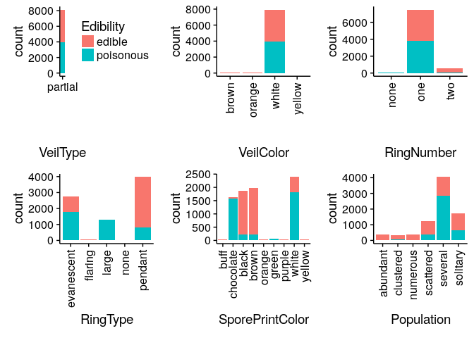
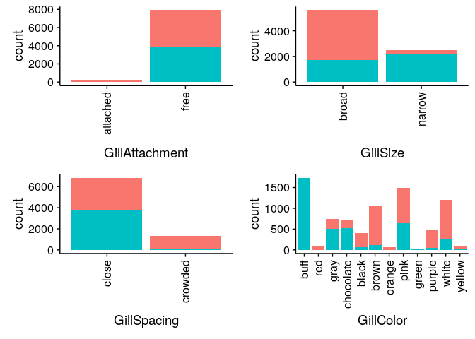
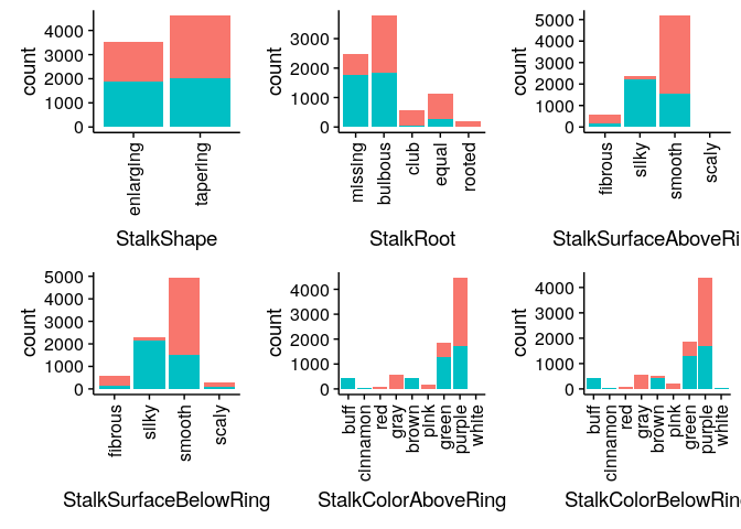
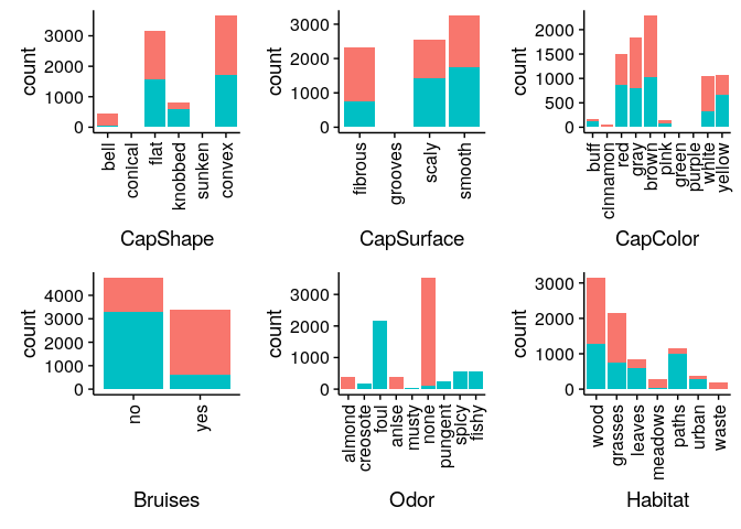
Bar Charts comparing Edibility across all mushroom features
Classifying Mushrooms:
Creating Train Test Splits
I will take 70% (5386 mushrooms) sample data for training & 30% (2438 mushrooms) for testing.
set.seed(2)
s=sample(1:nrow(mushroom),0.7*nrow(mushroom))
mush_train=mushroom[s,]
mush_test=mushroom[-s,]
mush_test1<- mush_test[, -1]
Creating Model using Naive Bayes Classifier
Naive Bayes classifier is based on Bayes Theorem with an assumption of independence among predictors. In simple terms, a Naive Bayes classifier assumes that the presence of a particular feature in a class is unrelated to the presence of any other feature.
model <- naiveBayes(Edibility ~. , data = mush_train)
Predicting Mushroom Class on Testset
Lets test our model on remaining 30% test data
pred <- predict(model, mush_test1)
Model Evaluation
confusionMatrix(pred,mush_test$Edibility)

## Confusion Matrix and Statistics
##
##            Reference
## Prediction  edible poisonous
##   edible      1245       147
##   poisonous      9      1037
##
##                Accuracy : 0.936
##                  95% CI : (0.9256, 0.9454)
##     No Information Rate : 0.5144
##     P-Value [Acc > NIR] : < 2.2e-16
##
##                   Kappa : 0.8715
##  Mcnemar's Test P-Value : < 2.2e-16
##
##             Sensitivity : 0.9928
##             Specificity : 0.8758
##          Pos Pred Value : 0.8944
##          Neg Pred Value : 0.9914
##              Prevalence : 0.5144
##          Detection Rate : 0.5107
##    Detection Prevalence : 0.5710
##       Balanced Accuracy : 0.9343
##
##        'Positive' Class : edible
##
In case of mushroom classification few False Negatives are tolerable but even a single False Positive can take someones life. We measure these as Sensitivity & Specificity.
We are getting Sensitivity(True Positive Rate) of 99.28% which is good as it represent our prediction for edible mushrooms & only .7% False negatives(9 Mushrooms).
But Specificity(True Negative Rate) or our ability to classify Poisonous mushrooms is 87.58%, which is not so good as more then 10% Poisonous mushrooms may get identified as Edible. This model have 147 False Positives which is not acceptable. so lets try a decision tree based model now.
Creating a Decision Tree based Classifier
Decision tree is a type of supervised learning algorithm works for both categorical and continuous input and output variables. In this technique, we split the population or sample into two or more homogeneous sets (or sub-populations) based on most significant splitter / differentiator in input variables.
tree.model <- rpart(Edibility ~ .,data = mush_train,method = "class",parms = list(split ="information"))
#prp(tree.model)
#summary(tree.model)
rpart.plot(tree.model,extra =  3,fallen.leaves = T)

tree.predict <- predict(tree.model, mush_test[,-c(1)], type = "class")
confusionMatrix(mush_test$Edibility, tree.predict)

## Confusion Matrix and Statistics
##
##            Reference
## Prediction  edible poisonous
##   edible      1254         0
##   poisonous     16      1168
##
##                Accuracy : 0.9934
##                  95% CI : (0.9894, 0.9962)
##     No Information Rate : 0.5209
##     P-Value [Acc > NIR] : < 2.2e-16
##
##                   Kappa : 0.9869
##  Mcnemar's Test P-Value : 0.0001768
##
##             Sensitivity : 0.9874
##             Specificity : 1.0000
##          Pos Pred Value : 1.0000
##          Neg Pred Value : 0.9865
##              Prevalence : 0.5209
##          Detection Rate : 0.5144
##    Detection Prevalence : 0.5144
##       Balanced Accuracy : 0.9937
##
##        'Positive' Class : edible
##
This model gives us an ideal Specificity of 1 but Decision Trees are prone to overfitting & so model may perform poorly on test data. Also algorithm have chosen only 2 attributes Order & SporePrintColor for making this prediction which might be questionable. Lets also try a final model called Random Forest which is robust & often gives a more generalizable model.
Creating Random Forest Classifier
Random forests are an ensemble learning method for classification, regression and other tasks, that operate by constructing a multitude of decision trees at training time and outputting the class that is the mode of the classes (classification) or mean prediction (regression) of the individual trees.
set.seed(1234)
rf_model <- randomForest(Edibility~.,data=mush_train, importance = TRUE, ntree = 1000)
rf_model

##
## Call:
##  randomForest(formula = Edibility ~ ., data = mush_train, importance = TRUE,      ntree = 1000)
##                Type of random forest: classification
##                      Number of trees: 1000
## No. of variables tried at each split: 4
##
##         OOB estimate of  error rate: 0%
## Confusion matrix:
##           edible poisonous class.error
## edible      2954         0           0
## poisonous      0      2732           0

varImpPlot(rf_model)
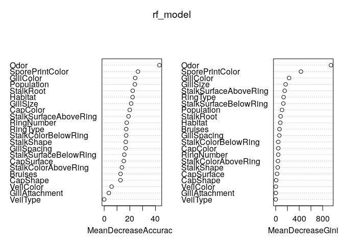
Random forest of 1000 trees have also identified Odor & SporePrintColor as most important variables. Lets check its predictions on test data now.
rf_prediction <- predict(rf_model, mush_test[,-c(1)])
confusionMatrix(mush_test$Edibility, rf_prediction)

## Confusion Matrix and Statistics
##
##            Reference
## Prediction  edible poisonous
##   edible      1254         0
##   poisonous      0      1184
##
##                Accuracy : 1
##                  95% CI : (0.9985, 1)
##     No Information Rate : 0.5144
##     P-Value [Acc > NIR] : < 2.2e-16
##
##                   Kappa : 1
##  Mcnemar's Test P-Value : NA
##
##             Sensitivity : 1.0000
##             Specificity : 1.0000
##          Pos Pred Value : 1.0000
##          Neg Pred Value : 1.0000
##              Prevalence : 0.5144
##          Detection Rate : 0.5144
##    Detection Prevalence : 0.5144
##       Balanced Accuracy : 1.0000
##
##        'Positive' Class : edible
##
We are getting 100% Accuracy, Sensitivity & Specificity now. I am not
sure if this is correct. Please share your feedback on errors &
improvements. Thanks for reading this notebook.